The proc_freq() function simulates a SAS® PROC FREQ
procedure. Below is a short tutorial on the function. Like PROC FREQ,
the function is both an interactive function and returns datasets.
Create Sample Data
The first step in our tutorial is to create some sample data:
# Create sample data
dat <- read.table(header = TRUE,
                  text = 'x y z
                          6 A 60
                          6 A 70
                          2 A 100
                          2 B 10
                          3 B 67
                          2 C 81
                          3 C 63
                          5 C 55')

# View sample data
dat
#   x y   z
# 1 6 A  60
# 2 6 A  70
# 3 2 A 100
# 4 2 B  10
# 5 3 B  67
# 6 2 C  81
# 7 3 C  63
# 8 5 C  55
Get Frequencies
Now that we have some data, let’s send that data to the
proc_freq() function to see the frequency distribution.
The options() statement below turns off printing of all
procs functions. This statement is necessary so that
the sample code below can pass CRAN checks. When running sample code
yourself, the options statement can be omitted.
# Turn off printing for CRAN
options("procs.print" = FALSE)
# Get frequencies
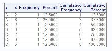
proc_freq(dat, tables = y)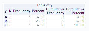
The above code illustrates a one-way frequency on the “y” variable. The result shows that the “A” and “C” categories appears three times, and the “B” category appears twice. The “N” column shows that there are eight items in the population. This population is used to get the percent shown for each frequency count.
Control Columns
The options parameter can control many aspects of the
proc_freq() function. For example, if you did not want the
cumulative frequency and percent, you could turn off these columns with
the option “nocum”.
# Turn off cumulative columns
proc_freq(dat, tables = y, options = nocum)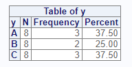
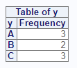
Let’s say you wanted only the frequency counts, and not the other
columns. This result can be achieved with the following options. Use the
v() function when you are passing multiple options:
Cross Tabulation
For two-way frequencies, you can cross two variables on the
tables parameter. This syntax produces a cross-tabulation
table by default:
# Create crosstab
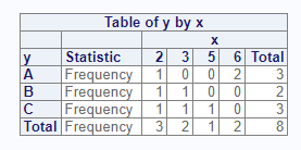
proc_freq(dat, tables = y * x)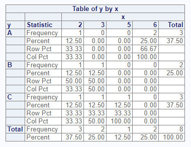
Cross Tabulation Options
If you want the data displayed in a list instead of a cross-tabulation table, you can do that with the “list” option. The “nosparse” option will turn off zero-count categories, which are included by default:
The following options turn off various features of the cross-tabulation table:
Multiple Tables
The tables parameter accepts more than one table
request. To request multiple tables, pass a quoted or unquoted vector.
Note that proc_freq() does not accept grouping syntax, such
as that allowed by SAS®. You must specify each cross-tab
individually:
# Request two crosstabs
proc_freq(dat, tables = v(y * x, y * z),
          options = v(norow, nocol, nopercent))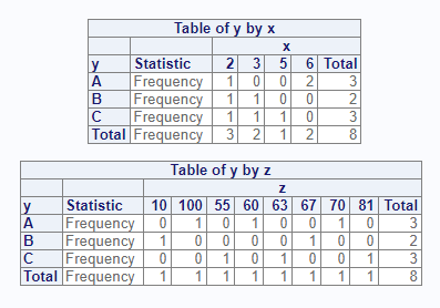
Distinct Values
The “nlevels” option can be used to count the number of distinct values in a categorical variable:
# Turn on nlevels option
proc_freq(dat, tables = y, options = nlevels)
<img src=“../man/images/freqtut8.png”, alt=“nlevels option” alt = “Proc freq distinct values”/>
Weighted Frequencies
The weight parameter is used to achieve weighted
frequencies. When a weight is specified, proc_freq() will
use the counts in the indicated variable for all frequency
calculations.
# Add weight variable
proc_freq(dat, tables = y, weight = z)
#   VAR CAT   N CNT      PCT
# 1   y   A 506 230 45.45455
# 2   y   B 506  77 15.21739
# 3   y   C 506 199 39.32806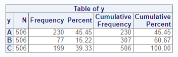
Where Expression
The where parameter can be used to filter the incoming
data before performing frequency counts. This parameter provides some
convenience when manipulating data. The parameter uses an
expression function that accepts non-standard evaluation
and any kind of R function or operator. Here is the above analysis, with
some values filtered out by the where expression:
# Add weight variable
proc_freq(dat, tables = y, weight = z,
          where = expression(z < 100))
#   VAR CAT   N CNT      PCT
# 1   y   A 406 130 32.01970
# 2   y   B 406  77 18.96552
# 3   y   C 406 199 49.01478
Statistics Options
The options parameter also accepts statistics options.
For two-way tables, you may request either Chi-Square or Fisher’s tests
of association. Here is an example of the Chi-Square test:
# Request Chi-Square and Output datasets
res <- proc_freq(dat, tables = y * x, options = chisq)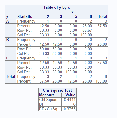
# View results
res
# $`y * x`
#    VAR1 VAR2 CAT1 CAT2 N CNT  PCT
# 1     y    x    A    2 8   1 12.5
# 2     y    x    A    3 8   0  0.0
# 3     y    x    A    5 8   0  0.0
# 4     y    x    A    6 8   2 25.0
# 5     y    x    B    2 8   1 12.5
# 6     y    x    B    3 8   1 12.5
# 7     y    x    B    5 8   0  0.0
# 8     y    x    B    6 8   0  0.0
# 9     y    x    C    2 8   1 12.5
# 10    y    x    C    3 8   1 12.5
# 11    y    x    C    5 8   1 12.5
# 12    y    x    C    6 8   0  0.0
#
# $`chisq:y * x`
#                         STAT DF      VAL      PROB
# 1                 Chi-Square  6 6.444444 0.3752853
# 2 Continuity Adj. Chi-Square  6 6.444444 0.3752853
Output Datasets
You may control datasets returned from the proc_freq()
function using the output parameter. This parameter takes
three basic values: “out”, “report”, and “none”. The “out” keyword
requests datasets meant for output, and is the default. These datasets
have standardized column names, and sometimes have additional columns to
help with data manipulation. The “report” keyword requests the exact
datasets used to create the interactive report. For both keywords, if
there is more than one dataset, they will be returned as a list of
datasets. The name of the list item will identify the dataset. You may
specify the names of the output tables in the list by using a named
table request.
Here is an example of the “out” option:
# Request output data
res <- proc_freq(dat, tables = v(x, y, MyCross = y * x),
                 output = out)

# View results
res
$x
  VAR CAT N CNT  PCT
1   x   2 8   3 37.5
2   x   3 8   2 25.0
3   x   5 8   1 12.5
4   x   6 8   2 25.0

$y
  VAR CAT N CNT  PCT
1   y   A 8   3 37.5
2   y   B 8   2 25.0
3   y   C 8   3 37.5

$MyCross
   VAR1 VAR2 CAT1 CAT2 N CNT  PCT
1     y    x    A    2 8   1 12.5
2     y    x    A    3 8   0  0.0
3     y    x    A    5 8   0  0.0
4     y    x    A    6 8   2 25.0
5     y    x    B    2 8   1 12.5
6     y    x    B    3 8   1 12.5
7     y    x    B    5 8   0  0.0
8     y    x    B    6 8   0  0.0
9     y    x    C    2 8   1 12.5
10    y    x    C    3 8   1 12.5
11    y    x    C    5 8   1 12.5
12    y    x    C    6 8   0  0.0
Notice that the way output datasets are requested from the
proc_freq() function is much simpler than the corresponding
mechanism in SAS®. With proc_freq(), by default, all
requested tables and statistics will be returned in a list. No other
output parameters are needed.
Output Ordering
The order parameter allows the user to control the sort
order of the outputs from proc_freq(). The possible
order values are “internal”, “data”, “freq”, and
“formatted”. These choices align with the corresponding procedure from
SAS. What is different with proc_freq() is that the
ordering applies to both the interactive report and the data frame
output.
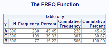
Let’s illustrate by taking the weighted frequency example from above, and request an order by frequency counts.
# Order by frequency counts
res <- proc_freq(dat,
                 tables = y,
                 weight = z,
                 order = freq)

# View return data frame
# Ordered by frequencies
res
#   VAR CAT   N CNT      PCT
# 1   y   A 506 230 45.45455
# 2   y   C 506 199 39.32806
# 3   y   B 506  77 15.21739
Notice how the output table is ordered by frequency count instead of the alphabetical value of “CAT”, which is the default.
The interactive report shows the same ordering:
The order parameter gives you control over the sort
order of proc_freq() results, which can help streamline the
processing of your data. Yet proc_freq() contains still
more capabilities to streamline the processing of your data.
Data Shaping
The proc_freq() function provides three options for
shaping data: “wide”, “long”, and “stacked”. These options control how
the output data is organized. The options are also passed on the
output parameter. The shaping options are best illustrated
by an example:
# Shape wide
res1 <- proc_freq(dat, tables = y,
                  output = wide)

# Wide results
res1
#   VAR CAT N CNT  PCT
# 1   y   A 8   3 37.5
# 2   y   B 8   2 25.0
# 3   y   C 8   3 37.5

# Shape long
res2 <- proc_freq(dat, tables = y,
                  output = long)

# Long results
res2
#   VAR STAT    A  B    C
# 1   y    N  8.0  8  8.0
# 2   y  CNT  3.0  2  3.0
# 3   y  PCT 37.5 25 37.5

# Shape stacked
res3 <- proc_freq(dat, tables = y,
                  output = stacked)

# Stacked results
res3
#   VAR CAT STAT VALUES
# 1   y   A    N    8.0
# 2   y   A  CNT    3.0
# 3   y   A  PCT   37.5
# 4   y   B    N    8.0
# 5   y   B  CNT    2.0
# 6   y   B  PCT   25.0
# 7   y   C    N    8.0
# 8   y   C  CNT    3.0
# 9   y   C  PCT   37.5
As seen above, the “wide” option places the statistics in columns across the top of the dataset and the categories in rows. This shaping option is the default. The “long” option places the statistics in rows, with each category in columns. The “stacked” option places both the statistics and the categories in rows.
These shaping options reduce some of the manipulation needed to get your data in the desired form. These options were added for convenience during the development of the procs package, and have no equivalent in SAS®.
Frequency Plots
To better understand your data, it is valuable to visualize it. The
proc_freq() function offers basic plotting of frequencies
via the “plots” parameter and the freqplot() function.
Default Plots
Here is a simple example demonstrating how to get default frequency plots for a selection of tables using the sample data from above:
proc_freq(dat, tables = v(x, y, x * y),
          weight = z,
          plots = TRUE)
The generated report will look like this:
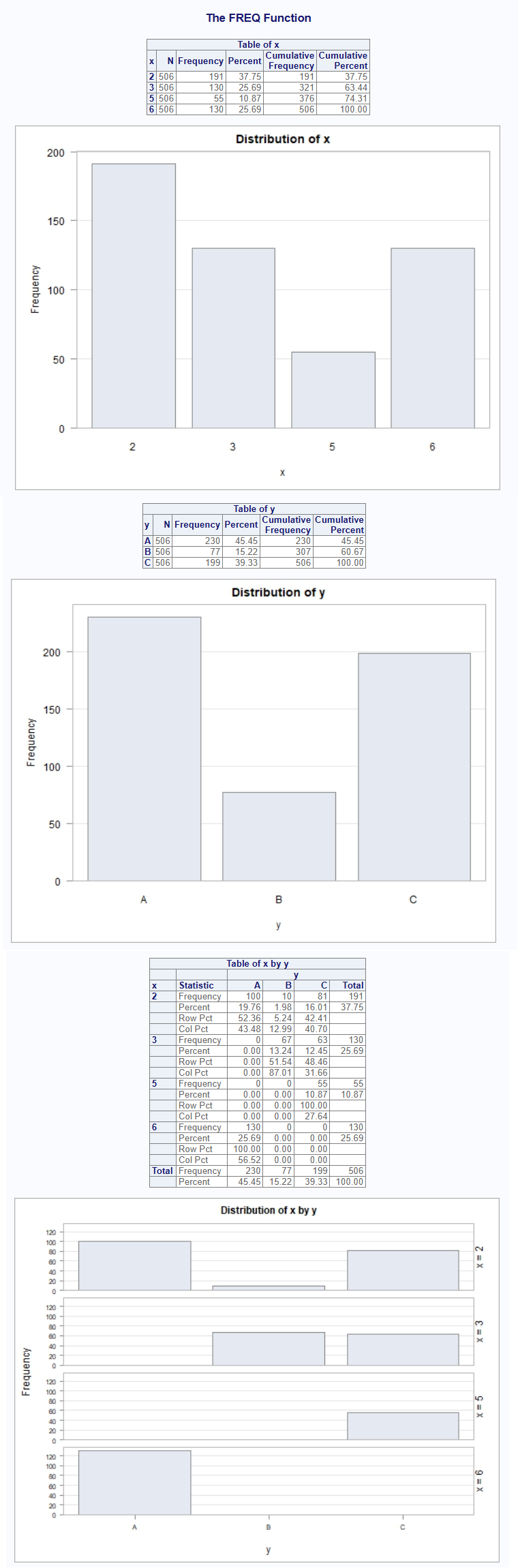
The report now shows a bar chart for each of the table requests. Note that on the two-way interaction, a bar chart is produced for each interaction and placed onto a single panel. If the interactions do not fit on a single panel, additional panels will be generated.
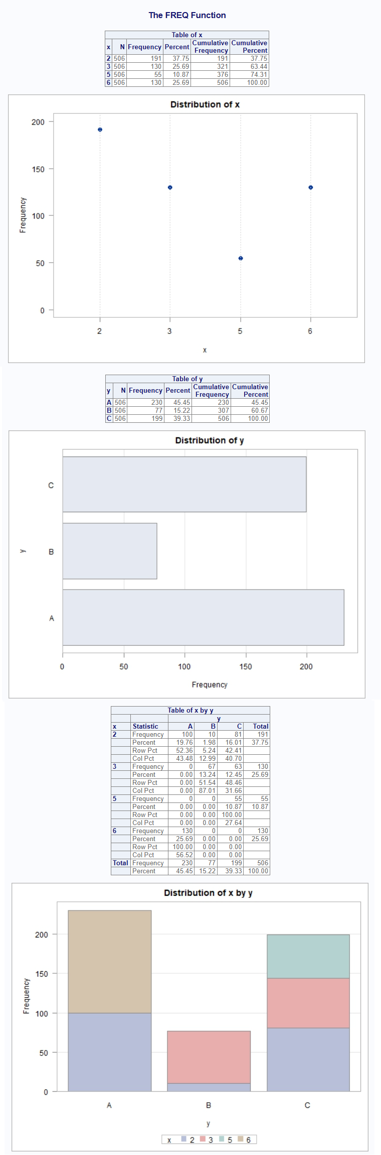
Customized Plots
The plots parameter on proc_freq() also
accepts a freqplot() object. This object offers some
customization of the requested plots. Besides the default frequency
chart produced in the example above, you may also request dot plots,
stacked bar charts, or clustered bar charts. The freqplot()
function also allows you to control the chart’s orientation, scale, and
other basic aspects of the plot.
If your call to proc_freq() has multiple tables, you can
pass a single freqplot() object that applies to all tables.
You may also customize the charts for each table in the
proc_freq() call. To customize the charts for each table,
pass separate calls to freqplot() in list, like this:
proc_freq(dat, tables = v(x, y, x * y),
          weight = z,
          plots = list(freqplot(type = "dotplot"),
                       freqplot(orient = "horizontal"),
                       freqplot(twoway = "stacked")))
Modifying the freqplot() parameters can help improve the
quality of your chart, and make it easier to understand what is
happening with your data. See the freqplot() documentation
for more information on how to customize your frequency plots.
Next: The Means Function