The proc_ttest() function simulates some of the
functionality of SAS® PROC TTEST. It can compute T-Tests and confidence
limits for one sample, paired samples, and two independent samples. The
function is both interactive and returns a list of data frames that can
be used for further analysis or reporting.
Create Sample Data
For the one and two sample T-Tests, we will use the following data.
This sample data is identical to the sashelp.class
dataset:
# Create sample data
cls <- read.table(header = TRUE, text = '
    Name Sex Age Height Weight
  Alfred   M  14   69.0  112.5
  Alice    F  13   56.5   84.0
  Barbara  F  13   65.3   98.0
  Carol    F  14   62.8  102.5
  Henry    M  14   63.5  102.5
  James    M  12   57.3   83.0
  Jane     F  12   59.8   84.5
  Janet    F  15   62.5  112.5
  Jeffrey  M  13   62.5   84.0
  John     M  12   59.0   99.5
  Joyce    F  11   51.3   50.5
  Judy     F  14   64.3   90.0
  Louise   F  12   56.3   77.0
  Mary     F  15   66.5  112.0
  Philip   M  16   72.0  150.0
  Robert   M  12   64.8  128.0
  Ronald   M  15   67.0  133.0
  Thomas   M  11   57.5   85.0
  William  M  15   66.5  112.0')
One Sample T-Test
A one-sample T-Test is used to determine if the mean of the target
variable is significantly different from a baseline or null hypothesis.
To perform this test, the target variable is passed on the
var parameter, and the null hypothesis is passed as an
option. Like this:
# Turn off printing to pass CRAN checks
options("procs.print" = FALSE)

# Single sample test
res1 <- proc_ttest(cls, var = Height, options = c(h0 = 65))

# View results
res1
# $Statistics
#      VAR  N     MEAN      STD   STDERR  MIN MAX
# 1 Height 19 62.33684 5.127075 1.176232 51.3  72
#
# $ConfLimits
#      VAR     MEAN     LCLM     UCLM      STD  LCLMSTD  UCLMSTD
# 1 Height 62.33684 59.86567 64.80801 5.127075 3.874083 7.582045
#
# $TTests
#      VAR DF         T      PROBT
# 1 Height 18 -2.264144 0.03615222
Observe that the results of the function is a list of three data frames: “Statistics”, “ConfLimits”, and “TTests”. If working in RStudio and printing is enabled, these same three result sets will be sent to the viewer:
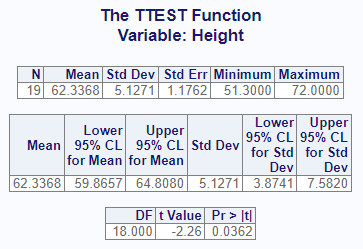
The interactive report allows you to quickly get a snapshot of statistical values for your data, and can help you determine the next course of action.
Two Sample T-Test
Now let’s test two independent samples. To test two independent
samples, the target variable is passed on the var parameter
as above. But the variable is split into two groups, as identified by
the variable on the class parameter. Here we will perform
another analysis on “Height”, and attempt to determine if there is a
significant difference between Males and Females with respect to
height:
# Perform two-sample analysis
res2 <- proc_ttest(cls, var = Height, class = Sex)

# View results
res2
# $Statistics
#      VAR      CLASS        METHOD  N      MEAN      STD   STDERR  MIN  MAX
# 1 Height          F          <NA>  9 60.588889 5.018328 1.672776 51.3 66.5
# 2 Height          M          <NA> 10 63.910000 4.937937 1.561513 57.3 72.0
# 3 Height Diff (1-2)        Pooled NA -3.321111       NA 2.286282   NA   NA
# 4 Height Diff (1-2) Satterthwaite NA -3.321111       NA 2.288340   NA   NA
#
# $ConfLimits
#      VAR      CLASS        METHOD      MEAN      LCLM      UCLM      STD  LCLMSTD  UCLMSTD
# 1 Height          F          <NA> 60.588889 56.731461 64.446317 5.018328 3.389665 9.613966
# 2 Height          M          <NA> 63.910000 60.377613 67.442387 4.937937 3.396487 9.014748
# 3 Height Diff (1-2)        Pooled -3.321111 -8.144744  1.502522       NA       NA       NA
# 4 Height Diff (1-2) Satterthwaite -3.321111 -8.155098  1.512875       NA       NA       NA
#
# $TTests
#      VAR        METHOD VARIANCES       DF         T     PROBT
# 1 Height        Pooled     Equal 17.00000 -1.452625 0.1645363
# 2 Height Satterthwaite   Unequal 16.72695 -1.451319 0.1651880
#
# $Equality
#      VAR   METHOD NDF DDF     FVAL     PROBF
# 1 Height Folded F   8   9 1.032825 0.9526904
The interactive output looks like this:
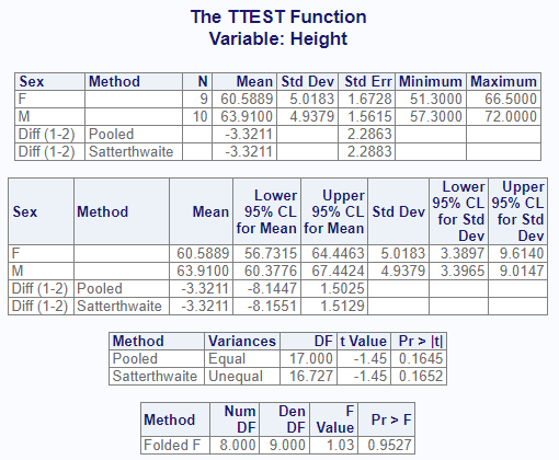
Notice that the output of the two independent variable T-Test is different than the single variable T-Test. The two variable T-Test provides separate descriptive statistics for the “Pooled” or “Satterthwaite” methods, and an additional “Equality” dataset that contains the F-Value. This additional information can help you interpret the T-Test results correctly.
Paired T-Test
For the paired T-Test, we will use the following data:
# Create sample data
paird <- read.table(header = TRUE, text = '
id before after
1 12 15
2 14 16
3 10 11
4 15 18
5 18 20
6 20 22
7 11 12
8 13 14
9 16 17
10 9 13')
To perform a paired T-Test, we use the paired parameter
on the proc_ttest() function, like so:
# Perform paired analysis
res3 <- proc_ttest(paird, paired = "before * after")

# View results
res3
# $Statistics
#     VAR1  VAR2         DIFF  N MEAN      STD    STDERR MIN MAX
# 1 before after before-after 10   -2 1.054093 0.3333333  -4  -1
#
# $ConfLimits
#     VAR1  VAR2         DIFF MEAN      LCLM      UCLM      STD  LCLMSTD  UCLMSTD
# 1 before after before-after   -2 -2.754052 -1.245948 1.054093 0.725042 1.924362
#
# $TTests
#     VAR1  VAR2         DIFF DF  T        PROBT
# 1 before after before-after  9 -6 0.0002024993
Here is the interactive report:
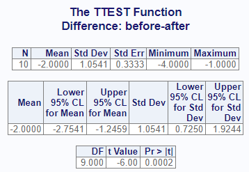
The paired analysis is used when you have some sort of natural relationship between the variables. Note that the procs T-Test function does not support shortcut syntax like parenthesis or hyphens like the SAS® PROC TTEST procedure. If you want to perform the paired analysis on multiple variables, pass them in a vector of strings.
By Groups
The proc_ttest() function provides a grouping parameter:
by. The by parameter identifies a variable or
variables for subsetting the input data. Here is the single sample
analysis shown above, but using the by parameter to perform
separate tests for Males and Females:
# By grouping
res5 <- proc_ttest(cls, var = "Height",
by = "Sex", options = c(h0 = 65))
# View Results
res5
# $Statistics
# BY VAR N MEAN STD STDERR MIN MAX
# 1 F Height 9 60.58889 5.018328 1.672776 51.3 66.5
# 2 M Height 10 63.91000 4.937937 1.561513 57.3 72.0
#
# $ConfLimits
# BY VAR MEAN LCLM UCLM STD LCLMSTD UCLMSTD
# 1 F Height 60.58889 56.73146 64.44632 5.018328 3.389665 9.613966
# 2 M Height 63.91000 60.37761 67.44239 4.937937 3.396487 9.014748
#
# $TTests
# BY VAR DF T PROBT
# 1 F Height 8 -2.637001 0.02985198
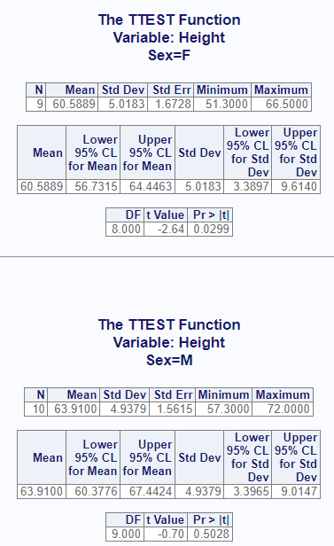
# 2 M Height 9 -0.698041 0.50278618For the interactive report, the by groups will be separated onto their own page:
Output Datasets
By default, the proc_ttest() function returns datasets.
Whether and what datasets the function returns are controlled by the
output parameter. There are three primary options: “out”,
“report”, and “none”. The “out” option is the default and returns
datasets meant for further manipulation and analysis. The “report”
keyword requests the exact datasets used in the interactive report. The
“none” keyword indicates that you don’t want any datasets returned. In
this case, the function will return a NULL.
We can see this difference by redoing the above paired T-Test with the “report” output option.
# Output dataset using "report" option
res4 <- proc_ttest(paird,
                   paired = "before * after",
                   output = "report")

# View results
res4
# $`diff1:Statistics`
#    N MEAN      STD    STDERR MIN MAX
# 1 10   -2 1.054093 0.3333333  -4  -1
#
# $`diff1:ConfLimits`
#   MEAN      LCLM      UCLM      STD  LCLMSTD  UCLMSTD
# 1   -2 -2.754052 -1.245948 1.054093 0.725042 1.924362
#
# $`diff1:TTests`
#   DF  T        PROBT
# 1  9 -6 0.0002024993
As can be seen in the above example, the “report” dataset contains fewer identifying variables than the default “out” dataset. The default datasets are generally more useful than the report datasets. Nevertheless, there may be times when you want to output the report datasets. For these times, the “report” output option is conveniently available.
Data Shaping
The “output” parameter may also be used to shape the data. There are three shaping options: “wide”, “long”, and “stacked”. The default is “wide”, and contains the statistics in columns and variables in rows.
Let’s use the single variable analysis with two variables to examine the “wide”, “long” and “stacked” shaping options. By running each option with the same analysis, we will be able to see the differences in the the output datasets clearly:
# Output option "wide"
res5 <- proc_ttest(cls, var = c("Height", "Weight"),
                   options = c(h0 = 65),
                   output = "wide")

# View results
res5
# $Statistics
#      VAR  N      MEAN       STD   STDERR  MIN MAX
# 1 Height 19  62.33684  5.127075 1.176232 51.3  72
# 2 Weight 19 100.02632 22.773933 5.224699 50.5 150
#
# $ConfLimits
#      VAR      MEAN     LCLM      UCLM       STD   LCLMSTD   UCLMSTD
# 1 Height  62.33684 59.86567  64.80801  5.127075  3.874083  7.582045
# 2 Weight 100.02632 89.04963 111.00300 22.773933 17.208272 33.678652
#
# $TTests
#      VAR DF         T        PROBT
# 1 Height 18 -2.264144 3.615222e-02
# 2 Weight 18  6.703988 2.754086e-06

# Output option "long"
res6 <- proc_ttest(cls, var = c("Height", "Weight"),
                   options = c(h0 = 65),
                   output = "long")

# View results
res6
# $Statistics
#     STAT    Height     Weight
# 1      N 19.000000  19.000000
# 2   MEAN 62.336842 100.026316
# 3    STD  5.127075  22.773933
# 4 STDERR  1.176232   5.224699
# 5    MIN 51.300000  50.500000
# 6    MAX 72.000000 150.000000
#
# $ConfLimits
#      STAT    Height    Weight
# 1    MEAN 62.336842 100.02632
# 2    LCLM 59.865671  89.04963
# 3    UCLM 64.808013 111.00300
# 4     STD  5.127075  22.77393
# 5 LCLMSTD  3.874083  17.20827
# 6 UCLMSTD  7.582045  33.67865
#
# $TTests
#    STAT      Height       Weight
# 1    DF 18.00000000 1.800000e+01
# 2     T -2.26414390 6.703988e+00
# 3 PROBT  0.03615222 2.754086e-06

# Output option "stacked"
res7 <- proc_ttest(cls, var = c("Height", "Weight"),
                   options = c(h0 = 65),
                   output = "stacked")

# View results
res7
# $Statistics
#       VAR   STAT     VALUES
# 1  Height      N  19.000000
# 2  Height   MEAN  62.336842
# 3  Height    STD   5.127075
# 4  Height STDERR   1.176232
# 5  Height    MIN  51.300000
# 6  Height    MAX  72.000000
# 7  Weight      N  19.000000
# 8  Weight   MEAN 100.026316
# 9  Weight    STD  22.773933
# 10 Weight STDERR   5.224699
# 11 Weight    MIN  50.500000
# 12 Weight    MAX 150.000000
#
# $ConfLimits
#       VAR    STAT     VALUES
# 1  Height    MEAN  62.336842
# 2  Height    LCLM  59.865671
# 3  Height    UCLM  64.808013
# 4  Height     STD   5.127075
# 5  Height LCLMSTD   3.874083
# 6  Height UCLMSTD   7.582045
# 7  Weight    MEAN 100.026316
# 8  Weight    LCLM  89.049631
# 9  Weight    UCLM 111.003000
# 10 Weight     STD  22.773933
# 11 Weight LCLMSTD  17.208272
# 12 Weight UCLMSTD  33.678652
#
# $TTests
#      VAR  STAT        VALUES
# 1 Height    DF  1.800000e+01
# 2 Height     T -2.264144e+00
# 3 Height PROBT  3.615222e-02
# 4 Weight    DF  1.800000e+01
# 5 Weight     T  6.703988e+00
# 6 Weight PROBT  2.754086e-06
Plots
proc_ttest() can generate plots for all types of
T-tests. The plots are very easy to generate. You will use the
plots parameter to make plot requests, and these requests
can be accomplished in several ways:
-
plots = TRUE: A TRUE value will return a default
set of plots for
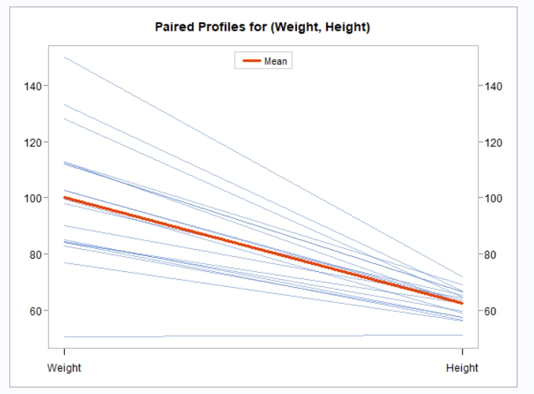
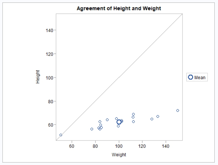
proc_ttest(). The default plots change depending on what type of analysis you are performing. All types of analysis include at least a summary distribution chart and a QQ plot. A paired analysis will also include a paired profiles chart and an agreement plot. - plots = “all”: The “all” keyword will return all available plots for the requested test.
-
plots = [vector of strings]: Plots may be requested
as a vector of plot names. These names are normally quoted, but may also
be passed unquoted using the
v()function. The available plot names are “agreement”, “boxplot”, “histogram”, “interval”, “profiles”, “qqplot”, and “summary”. -
plots = ttestplot([with parameters]): The
ttestplot()function gives you the most control over the charts produced. This function takes parameters which allow you to specify which charts to show, and some other customization features. See thettestplot()function for additional details.
Let’s re-run the one sample T-Test from above, but this time with
plots. In this case, we want to see the null hypothesis on the chart,
and request an interval chart in addition to the default summary and
qqplot. Therefore, we can perform a custom plot request with the
ttestplot() function and pass the desired parameters:
# One sample T-Test with plots
proc_ttest(cls, var = Height, options = c(h0 = 65),
           plots = ttestplot(c("summary", "qqplot", "interval"),
                             showh0 = TRUE))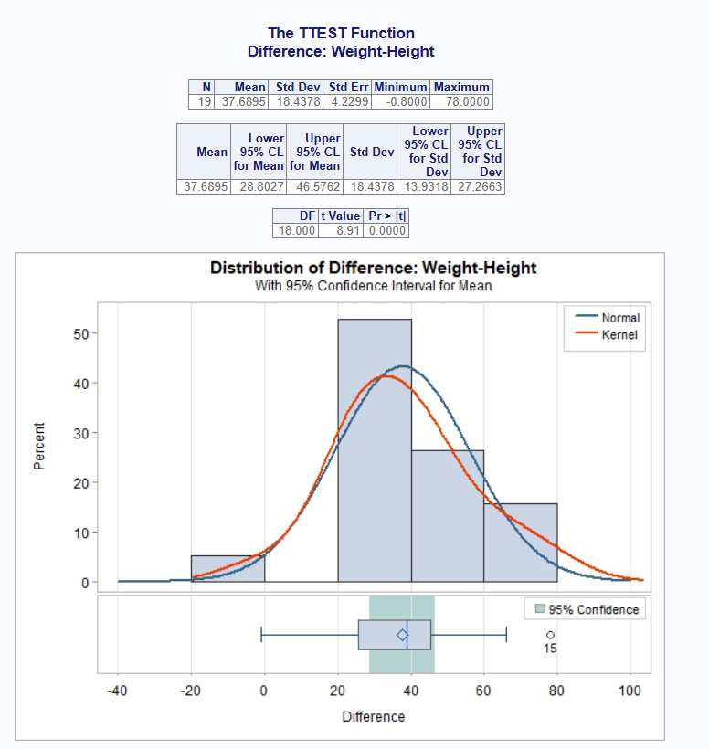
Notice the amount of analysis performed by a single call to
proc_ttest(). These functions are designed with needs of
the analyst in mind, and can give you an enormous amount of information
with very little effort.
Next: Regression Function