The procs package contains functions that replicate procedures from SAS® software. The intention of the package is to ease R adoption by providing SAS® programmers a familiar conceptual framework and functions that produce nearly identical output. Along the way, the functions in the procs package also provide much nicer output than many R statistical functions.
Key Functions
The package includes the following functions:
-
proc_freq(): A function to simulate the FREQ procedure. -
proc_means(): A function to simulate the MEANS or SUMMARY procedure. -
proc_ttest(): A function to perform T-Tests and calculate confidence limits. -
proc_reg(): A function to perform a regression. -
proc_transpose(): A function to pivot data similar in syntax to the TRANSPOSE procedure. -
proc_sort(): A function to sort and dedupe datasets. -
proc_print(): A quick-print function to send procedure results to the viewer or a report.
How to Use
Frequency Statistics
The proc_freq() function generates frequency statistics
in a manner similar to SAS® PROC FREQ. You can request one-way and
two-way frequency tables using the tables parameter.
Frequencies may be weighted using the weight parameter.
Simply pass the name of the variable that contains the weighted values.
There are many options to control the output data and display.
Note that the options("procs.print" = FALSE) global
option has been added to these examples to allow the
procs package to pass CRAN checks. When running sample
code yourself, remove this option or set it to TRUE.
library(procs)

# Turn off printing for CRAN checks
options("procs.print" = FALSE)

# Prepare sample data
dt <- as.data.frame(HairEyeColor, stringsAsFactors = FALSE)

# Assign labels
labels(dt) <- list(Hair = "Hair Color",
                   Eye = "Eye Color")

# Produce frequency statistics
res <- proc_freq(dt, tables = v(Hair, Eye, Hair * Eye),
                 weight = Freq,
                 output = report,
                 options = chisq,
                 titles = "Hair and Eye Frequency Statistics")
When printing is allowed, the proc_freq() function will
display the following report in the viewer: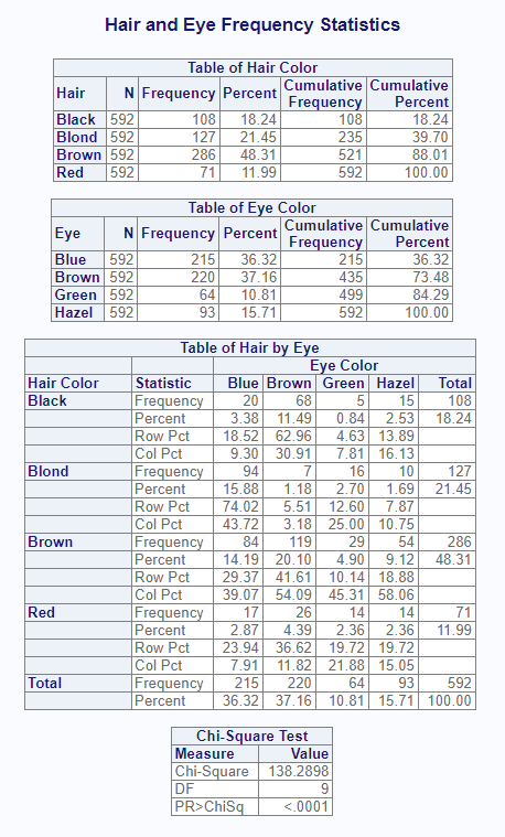
The function call requested output datasets using the “report” option. If there is more than one output dataset, they will be returned in a list. The output dataset list can be seen below:
# View output datasets
res
# $Hair
#     CAT   N CNT      PCT CUMSUM    CUMPCT
# 1 Black 592 108 18.24324    108  18.24324
# 2 Blond 592 127 21.45270    235  39.69595
# 3 Brown 592 286 48.31081    521  88.00676
# 4   Red 592  71 11.99324    592 100.00000
#
# $Eye
#     CAT   N CNT      PCT CUMSUM    CUMPCT
# 1  Blue 592 215 36.31757    215  36.31757
# 2 Brown 592 220 37.16216    435  73.47973
# 3 Green 592  64 10.81081    499  84.29054
# 4 Hazel 592  93 15.70946    592 100.00000
#
# $`Hair * Eye`
#      CAT Statistic       Blue      Brown      Green     Hazel     Total
# 1  Black Frequency  20.000000  68.000000  5.0000000 15.000000 108.00000
# 2  Black   Percent   3.378378  11.486486  0.8445946  2.533784  18.24324
# 3  Black   Row Pct  18.518519  62.962963  4.6296296 13.888889        NA
# 4  Black   Col Pct   9.302326  30.909091  7.8125000 16.129032        NA
# 5  Blond Frequency  94.000000   7.000000 16.0000000 10.000000 127.00000
# 6  Blond   Percent  15.878378   1.182432  2.7027027  1.689189  21.45270
# 7  Blond   Row Pct  74.015748   5.511811 12.5984252  7.874016        NA
# 8  Blond   Col Pct  43.720930   3.181818 25.0000000 10.752688        NA
# 9  Brown Frequency  84.000000 119.000000 29.0000000 54.000000 286.00000
# 10 Brown   Percent  14.189189  20.101351  4.8986486  9.121622  48.31081
# 11 Brown   Row Pct  29.370629  41.608392 10.1398601 18.881119        NA
# 12 Brown   Col Pct  39.069767  54.090909 45.3125000 58.064516        NA
# 13   Red Frequency  17.000000  26.000000 14.0000000 14.000000  71.00000
# 14   Red   Percent   2.871622   4.391892  2.3648649  2.364865  11.99324
# 15   Red   Row Pct  23.943662  36.619718 19.7183099 19.718310        NA
# 16   Red   Col Pct   7.906977  11.818182 21.8750000 15.053763        NA
# 17 Total Frequency 215.000000 220.000000 64.0000000 93.000000 592.00000
# 18 Total   Percent  36.317568  37.162162 10.8108108 15.709459 100.00000
#
# $Chisq
#                         STAT DF      VAL         PROB
# 1                 Chi-Square  9 138.2898 2.325287e-25
# 2 Continuity Adj. Chi-Square  9 138.2898 2.325287e-25
Summary Statistics
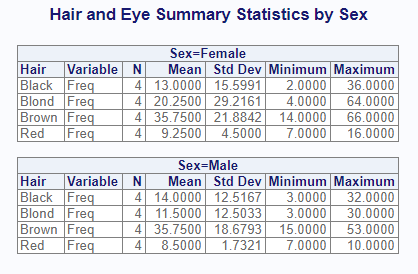
The proc_means() function calculates summary statistics,
similar to the SAS® PROC MEANS procedure. The variable or variables to
generate statistics for is passed on the var parameter. The
class parameter tells the function to group results by the
indicated variable. The by parameter will subset the data
according to the distinct by values. Note that any class groupings are
nested in the by.
# Perform calculations
res2 <- proc_means(dt, var = Freq,
                   class = Hair,
                   by = Sex,
                   options = c(maxdec = 4),
                   titles = "Hair and Eye Summary Statistics by Sex")
The following is sent to the viewer:
And here is the output dataset. Observe that the output dataset is not identical to the displayed report. The output dataset has been optimized for data manipulation, while the displayed report has been optimized for viewing:
# View the summary statistics
res2
#        BY CLASS TYPE FREQ  VAR  N    MEAN       STD MIN MAX
# 1  Female  <NA>    0   16 Freq 16 19.5625 20.713824   2  66
# 2  Female Black    1    4 Freq  4 13.0000 15.599145   2  36
# 3  Female Blond    1    4 Freq  4 20.2500 29.216149   4  64
# 4  Female Brown    1    4 Freq  4 35.7500 21.884165  14  66
# 5  Female   Red    1    4 Freq  4  9.2500  4.500000   7  16
# 6    Male  <NA>    0   16 Freq 16 17.4375 16.008201   3  53
# 7    Male Black    1    4 Freq  4 14.0000 12.516656   3  32
# 8    Male Blond    1    4 Freq  4 11.5000 12.503333   3  30
# 9    Male Brown    1    4 Freq  4 35.7500 18.679311  15  53
# 10   Male   Red    1    4 Freq  4  8.5000  1.732051   7  10
Notice that the output data contains breakouts by class and summaries by group. The summaries by group are identifed by rows where TYPE = 0. The breakouts by class are TYPE = 1. In other words, rows 1 and 6 provide summary statistics for the by groups FEMALE and MALE, while the other rows provide statistics for each class category.
Also note that both proc_freq() and
proc_means() output datasets follow the convention of
naming columns according to the statistic or parameter they represent.
This convention is somewhat different from SAS®, but makes it easier to
manipulate the output data.
Hypothesis Testing
Similar to PROC TTEST in SAS®, the proc_ttest() function
performs hypothesis testing and calculates confidence limits. The
function can operate on a single variable, two independent samples, or
paired observations.
The paired observation test can be used in cases when you have samples on the same measure at different time points, or before and after a procedure. This example attempts to determine whether there is a significant change in systolic blood pressure before and after a stimulus. It uses the following data:
# Create sample data
pressure <- read.table(header = TRUE, text = '
  SBPbefore SBPafter
  120 128
  124 131
  130 131
  118 127
  140 132
  128 125
  140 141
  135 137
  126 118
  130 132
  126 129
  127 135
  ')
Now let’s determine if there is a significant change before and after
the stimulus. For this type of T-Test test, we will use the
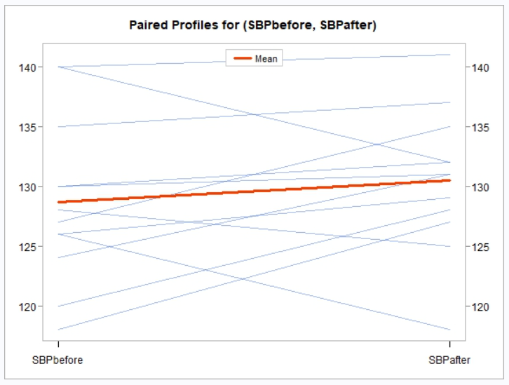
paired parameter. To better understand the data, we will
also turn on the default plots:
# Perform T-Test
res3 <- proc_ttest(pressure, paired = "SBPbefore * SBPafter",
                   plots = TRUE)

# View results
res3
# $Statistics
#                  VAR  N      MEAN      STD   STDERR MIN MAX
# 1 SBPbefore-SBPafter 12 -1.833333 5.828353 1.682501  -9   8
#
# $ConfLimits
#                  VAR      MEAN      LCLM     UCLM      STD
# 1 SBPbefore-SBPafter -1.833333 -5.536492 1.869825 5.828353
#
# $TTests
#                  VAR DF         T     PROBT
# 1 SBPbefore-SBPafter 11 -1.089648 0.2991635
If printing is enabled, the following is sent to the viewer:
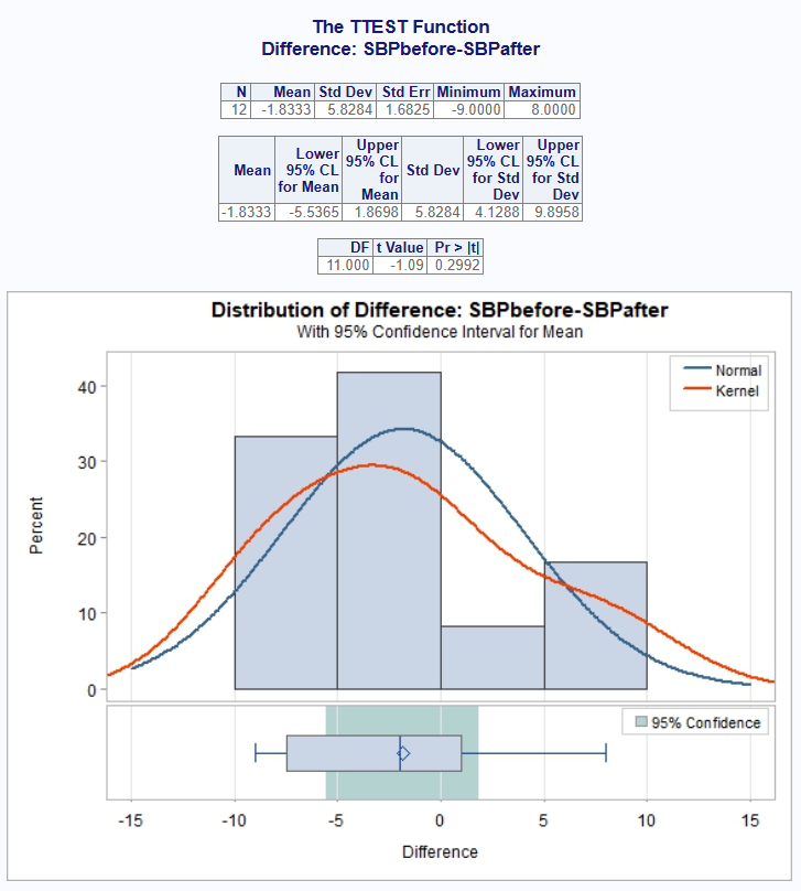
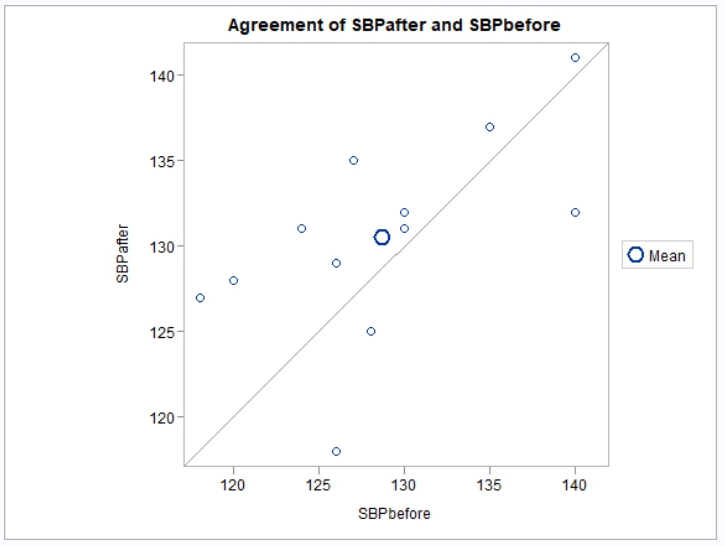
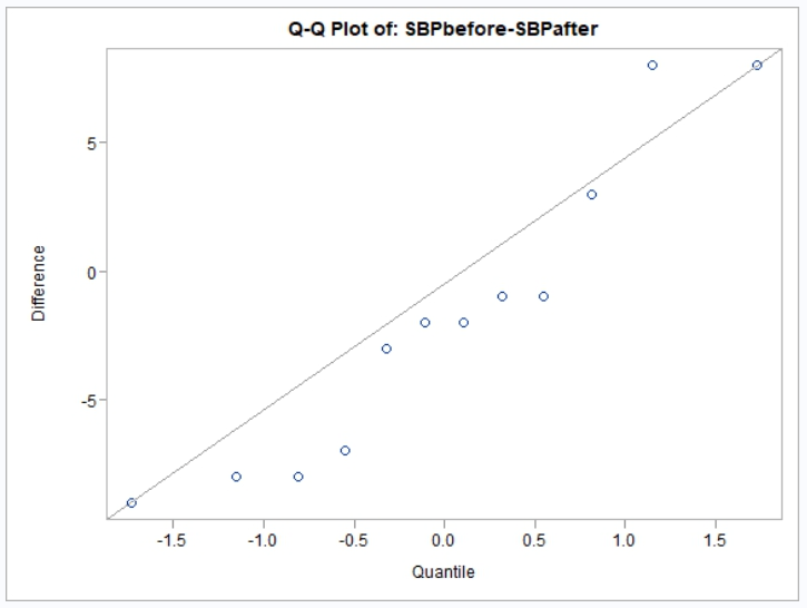
The above test shows although there was a change before and after the stimulus, that change was not statistically significant.
Note that the proc_freq() and proc_req()
functions also have the capability to generate plots for the selected
analysis. See the documentation of those functions for more details.
Other Functions
While the main focus of the procs package is on
statistical procedures, the output from these procedures is often
manipulated to produce a more desirable result. Some additional
functions have been added to the procs package that
SAS® programmers will be familiar with: proc_transpose(),
proc_sort(), and proc_print().
Continuing from the means example above, let’s take some additional steps to produce a little report:
library(fmtr)

# Filter and select using subset function
res4 <- subset(res2, TYPE != 0, c(BY, CLASS, N, MEAN, STD, MIN, MAX))

# Transpose statistics
res5 <- proc_transpose(res3, id = CLASS, by = BY, name = Statistic)

# View transformed data
res5
#        BY Statistic    Black    Blond    Brown       Red
# 1  Female         N  4.00000  4.00000  4.00000  4.000000
# 2  Female      MEAN 13.00000 20.25000 35.75000  9.250000
# 3  Female       STD 15.59915 29.21615 21.88416  4.500000
# 4  Female       MIN  2.00000  4.00000 14.00000  7.000000
# 5  Female       MAX 36.00000 64.00000 66.00000 16.000000
# 6    Male         N  4.00000  4.00000  4.00000  4.000000
# 7    Male      MEAN 14.00000 11.50000 35.75000  8.500000
# 8    Male       STD 12.51666 12.50333 18.67931  1.732051
# 9    Male       MIN  3.00000  3.00000 15.00000  7.000000
# 10   Male       MAX 32.00000 30.00000 53.00000 10.000000

# Assign factor to BY so we can sort
res5$BY <- factor(res5$BY, levels = c("Male", "Female"))

# Sort male to top
res6 <- proc_sort(res5, by = BY)
#        BY Statistic    Black    Blond    Brown       Red
# 6    Male         N  4.00000  4.00000  4.00000  4.000000
# 7    Male      MEAN 14.00000 11.50000 35.75000  8.500000
# 8    Male       STD 12.51666 12.50333 18.67931  1.732051
# 9    Male       MIN  3.00000  3.00000 15.00000  7.000000
# 10   Male       MAX 32.00000 30.00000 53.00000 10.000000
# 1  Female         N  4.00000  4.00000  4.00000  4.000000
# 2  Female      MEAN 13.00000 20.25000 35.75000  9.250000
# 3  Female       STD 15.59915 29.21615 21.88416  4.500000
# 4  Female       MIN  2.00000  4.00000 14.00000  7.000000
# 5  Female       MAX 36.00000 64.00000 66.00000 16.000000

# Create formatting list
fmt <- flist(STD = "%.3f", type = "row", lookup = res6$Statistic)

# Create vector lookup
vf <- c(MEAN = "Mean", STD = "Std", MEDIAN = "Median",
        MIN = "Min", MAX = "Max")

# Assign formats
formats(res6) <- list(Statistic = vf,
                      Black = fmt,
                      Blond = fmt,
                      Brown = fmt,
                      Red = fmt)

# Reassign first column name
names(res6)[1] <- "stub"

# Assign labels
labels(res6) <- list(stub = "Sex")

# Create list for reporting
prnt <- list(res$`Hair * Eye`, res$Chisq, res6)

# Print result
proc_print(prnt,
           titles = "Analysis of Hair and Eyes Dataset",
           view = FALSE) # Set view = TRUE to see results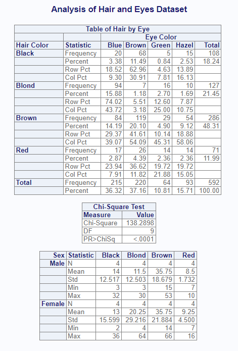
If desired, we could print this report to the file system using the
file_path and output_type parameters on
proc_print().