The proc_means() function simulates a SAS® PROC MEANS
procedure. It is used to generate summary statistics on numeric
variables. The function is both interactive and returns datasets.
Create Sample Data
Let’s again create some sample data. This sample data is identical to
that created for the proc_freq() tutorial, but has an
additional grouping variable “g”:
Get Summary Statistics
If no parameters are specified, the proc_means()
function will calculate N, Means, Standard Deviation, Minimum, and
Maximum on all numeric variables.
Note that the options statement has been added to pass
CRAN checks. When you are running code samples, this statement may be
omitted.
# Turn off printing for CRAN checks
options("procs.print" = FALSE)

# No parameters
proc_means(dat)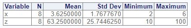
Selected Variables
If you don’t want statistics on all numeric variables, you may
specify variables on the var parameter:
# Specific variable
proc_means(dat, var = x)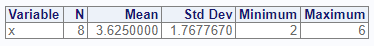
Statistics Options
The proc_means() function has a stats
parameter that allows you to control which statistics are generated.
There are many statistics keywords. Here is a sample of some of the most
frequently used keywords:
| Keyword | Description |
|---|---|
| N | Number of Observations |
| NMISS | Number of missing observations |
| MEAN | Arithmetic mean |
| STD | Standard Deviation |
| MIN | Minimum |
| MAX | Maximum |
| SUM | Sum of observations |
| MEDIAN | 50th percentile |
| P1 | 1st percentile |
| P5 | 5st percentile |
| P10 | 10th percentile |
| P90 | 90th percentile |
| P95 | 95th percentile |
| P99 | 99th percentile |
| Q1 | First Quartile |
| Q3 | Third Quartile |
Now that we know some statistics keywords, let’s practice using them. Here is an example which calculates the median, sum, first quartile, and third quartile for all numeric variables in our sample data:
# Custom statistics options
proc_means(dat, stats = v(median, sum, q1, q3))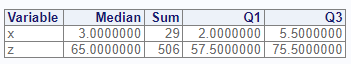
Output Datasets
Similar to the proc_freq() function,
proc_means() can return datasets. There are three options:
“out”, “report”, and “none”. The “out” option returns datasets meant for
further manipulation and analysis, and is the default. The “report”
keyword requests the exact datasets used in the interactive report.
Specifying either one of these options will cause the function to return
data.
Here is an example that shows the difference in the “report” and “out” options:
# Output dataset using "report" option
res1 <- proc_means(dat,
                   stats = v(median, sum, q1, q3),
                   output = report)

# View results
res1
#   VAR MEDIAN SUM   Q1   Q3
# 1   x      3  29  2.0  5.5
# 2   z     65 506 57.5 75.5


# Output dataset using "out" option
res2 <- proc_means(dat,
                   stats = v(median, sum, q1, q3),
                   output = out)

# View results
res2
#   TYPE FREQ VAR MEDIAN SUM   Q1   Q3
# 1    0    8   x      3  29  2.0  5.5
# 2    0    8   z     65 506 57.5 75.5
As can be seen in the above example, the “out” dataset includes additional variables for TYPE and FREQ. These additional variables can be turned off with options:
# Turn off TYPE and FREQ variables
res3 <- proc_means(dat,
                   stats = v(median, sum, q1, q3),
                   output = out,
                   options = v(notype, nofreq))

# View results
res3
#   VAR MEDIAN SUM   Q1   Q3
# 1   x      3  29  2.0  5.5
# 2   z     65 506 57.5 75.5
Grouping
The proc_means() function provides two grouping
parameters: class and by. These parameters
identify a variable or variables for subsetting the input data. While
these parameters have similar capabilities, there are some difference
between them. The differences can be examined by comparing the two
function calls.
Class
# Class grouping
res1 <- proc_means(dat, stats = v(median, sum, q1, q3),
                   class = y, options = v(maxdec = 4))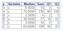
Below is the output dataset from the class parameter.
Notice that summary values have been provided for each variable, in
addition to the subsets by the class variable. The summary rows are
identifed by TYPE = 0, while the subset rows are TYPE = 1.
# View results - class
res1
#   CLASS TYPE FREQ VAR MEDIAN SUM   Q1    Q3
# 1  <NA>    0    8   x    3.0  29  2.0   5.5
# 2  <NA>    0    8   z   65.0 506 57.5  75.5
# 3     A    1    3   x    6.0  14  2.0   6.0
# 4     A    1    3   z   70.0 230 60.0 100.0
# 5     B    1    2   x    2.5   5  2.0   3.0
# 6     B    1    2   z   38.5  77 10.0  67.0
# 7     C    1    3   x    3.0  10  2.0   5.0
# 8     C    1    3   z   63.0 199 55.0  81.0
By
Here is the same analysis using the by parameter instead
of the class parameter:
# By grouping
res2 <- proc_means(dat, stats = v(median, sum, q1, q3),
                   by = y, options = v(maxdec = 4))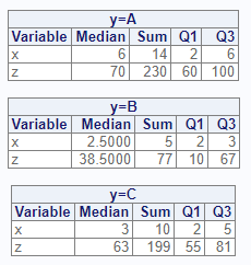
Notice that with the by parameter, separate tables are
created for each by group on the interactive report.
Now let’s look at the output dataset:
# View results - by
res2
#   BY TYPE FREQ VAR MEDIAN SUM Q1  Q3
# 1  A    0    3   x    6.0  14  2   6
# 2  A    0    3   z   70.0 230 60 100
# 3  B    0    2   x    2.5   5  2   3
# 4  B    0    2   z   38.5  77 10  67
# 5  C    0    3   x    3.0  10  2   5
# 6  C    0    3   z   63.0 199 55  81
The output dataset is also different from the class
output. While the TYPE variables exists on the output dataset, the
output data for the by group does not include the summary rows. The
summary rows are a feature of the class variable. You
should select the grouping parameter that most suits your needs.
Multiple Groups
Class
The proc_means() function can perform analysis with
multiple grouping variables. First let’s examine what happens when we
pass multiple grouping variables to the class
parameter:
# Class grouping - two variables
res1 <- proc_means(dat, stats = v(median, sum, q1, q3),
                   class = v(g, y), options = v(maxdec = 0))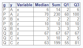
Here is the output dataset:
# View results - two class variables
res1
#    CLASS1 CLASS2 TYPE FREQ VAR MEDIAN SUM   Q1    Q3
# 1    <NA>   <NA>    0    8   x    3.0  29  2.0   5.5
# 2    <NA>   <NA>    0    8   z   65.0 506 57.5  75.5
# 3    <NA>      A    1    3   x    6.0  14  2.0   6.0
# 4    <NA>      A    1    3   z   70.0 230 60.0 100.0
# 5    <NA>      B    1    2   x    2.5   5  2.0   3.0
# 6    <NA>      B    1    2   z   38.5  77 10.0  67.0
# 7    <NA>      C    1    3   x    3.0  10  2.0   5.0
# 8    <NA>      C    1    3   z   63.0 199 55.0  81.0
# 9       P   <NA>    2    4   x    4.0  16  2.0   6.0
# 10      P   <NA>    2    4   z   65.0 240 35.0  85.0
# 11      Q   <NA>    2    4   x    3.0  13  2.5   4.0
# 12      Q   <NA>    2    4   z   65.0 266 59.0  74.0
# 13      P      A    3    3   x    6.0  14  2.0   6.0
# 14      P      A    3    3   z   70.0 230 60.0 100.0
# 15      P      B    3    1   x    2.0   2  2.0   2.0
# 16      P      B    3    1   z   10.0  10 10.0  10.0
# 17      Q      B    3    1   x    3.0   3  3.0   3.0
# 18      Q      B    3    1   z   67.0  67 67.0  67.0
# 19      Q      C    3    3   x    3.0  10  2.0   5.0
# 20      Q      C    3    3   z   63.0 199 55.0  81.0
Observe that the function produces statistics for each set of
combinations of the class variable. Each level of
combinations is identified by the TYPE value. To turn off the class
combinations, pass the “nway” option.
By
Now let’s see what happens when we use the by parameter
with two variables:
# By grouping - two variables
res2 <- proc_means(dat, stats = v(median, sum, q1, q3),
                   by = v(g, y), options = v(maxdec = 0))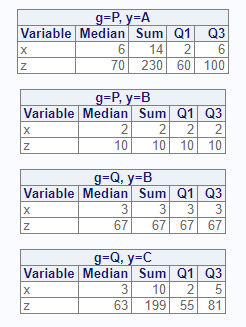
Here is the output dataset for the by parameter:
# View results - two by variables
res2
#   BY1 BY2 TYPE FREQ VAR MEDIAN SUM Q1  Q3
# 1   P   A    0    3   x      6  14  2   6
# 2   P   A    0    3   z     70 230 60 100
# 3   P   B    0    1   x      2   2  2   2
# 4   P   B    0    1   z     10  10 10  10
# 5   Q   B    0    1   x      3   3  3   3
# 6   Q   B    0    1   z     67  67 67  67
# 7   Q   C    0    3   x      3  10  2   5
# 8   Q   C    0    3   z     63 199 55  81
By and Class
Finally, let’s see what happens when we specify both by
and class parameters:
# By grouping - by and class
res3 <- proc_means(dat, stats = v(median, sum, q1, q3),
                   by = g,
                   class = y,
                   options = v(maxdec = 0))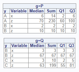
# View results - by and class
res3
#    BY CLASS TYPE FREQ VAR MEDIAN SUM   Q1  Q3
# 1   P  <NA>    0    4   x      4  16  2.0   6
# 2   P  <NA>    0    4   z     65 240 35.0  85
# 3   P     A    1    3   x      6  14  2.0   6
# 4   P     A    1    3   z     70 230 60.0 100
# 5   P     B    1    1   x      2   2  2.0   2
# 6   P     B    1    1   z     10  10 10.0  10
# 7   Q  <NA>    0    4   x      3  13  2.5   4
# 8   Q  <NA>    0    4   z     65 266 59.0  74
# 9   Q     B    1    1   x      3   3  3.0   3
# 10  Q     B    1    1   z     67  67 67.0  67
# 11  Q     C    1    3   x      3  10  2.0   5
# 12  Q     C    1    3   z     63 199 55.0  81
Weight
Sometimes you need to calculate statistics using the relative
importance of an observation. In these cases, proc_means()
allows the use of a weighted value for each observation. The weighted
value for an observation can be passed on the weight
parameter.
First, let’s create some data to use for our analysis:
dat2 <- read.table(header = TRUE, text = '
                Name      Assessment     Score   Weight
                Smith     Quiz1          84      0.05
                Smith     Quiz2          25      0.05
                Smith     Midterm        85      0.35
                Smith     Quiz3           0      0.05
                Smith     Quiz4          62      0.05
                Smith     Final          93      0.45
                Wang      Quiz1         100      0.05
                Wang      Quiz2          95      0.05
                Wang      Midterm        98      0.35
                Wang      Quiz3         105      0.05
                Wang      Quiz4          87      0.05
                Wang      Final          96      0.45')

# View data
dat2
#     Name Assessment Score Weight
# 1  Smith      Quiz1    84   0.05
# 2  Smith      Quiz2    25   0.05
# 3  Smith    Midterm    85   0.35
# 4  Smith      Quiz3     0   0.05
# 5  Smith      Quiz4    62   0.05
# 6  Smith      Final    93   0.45
# 7   Wang      Quiz1   100   0.05
# 8   Wang      Quiz2    95   0.05
# 9   Wang    Midterm    98   0.35
# 10  Wang      Quiz3   105   0.05
# 11  Wang      Quiz4    87   0.05
# 12  Wang      Final    96   0.45
To understand how the weighting works, let’s then calculate some un-weighted statistics on this data:
res <- proc_means(dat2, var = Score,
                  class = Name,
                  options = "nway",
                  stats = v(n, mean, median, std, min, max, vari))

# View results
res
#   CLASS TYPE FREQ   VAR N     MEAN MEDIAN       STD MIN MAX       VARI
# 1 Smith    1    6 Score 6 58.16667     73 37.679791   0  93 1419.76667
# 2  Wang    1    6 Score 6 96.83333     97  5.980524  87 105   35.76667
Now let’s use the weight parameter to calculate weighted
statistics:
res <- proc_means(dat2, var = Score,
                  class = Name,
                  weight = Weight,
                  options = c("nway", vardef = "wgt"),
                  stats = v(n, mean, median, std, min, max, vari))

# View results
res
#   CLASS TYPE FREQ   VAR N  MEAN MEDIAN       STD MIN MAX     VARI
# 1 Smith    1    6 Score 6 80.15     85 23.937993   0  93 573.0275
# 2  Wang    1    6 Score 6 96.85     96  3.102821  87 105   9.6275
Notice that the function returned weighted values for the mean, median, standard deviation, and variance. However, the statistics for n, min, and max did not change.
Also note that the “vardef” option controls which denominator is used
for the variance (VARI) statistic. See the proc_means()
documentation for further information on this option.
Where Expression
You can perform subsetting of the proc_means() data with
a where expression. To add a where expression, pass an
expression function to the where parameter.
For example, here is the above analysis with a where expression:
res <- proc_means(dat2, var = Score,
                  class = Name,
                  weight = Weight,
                  options = c("nway", vardef = "wgt"),
                  stats = v(n, mean, median, std, min, max, vari),
                  where = expression(Score <= 100)
                  )

# View results
res
#   CLASS TYPE FREQ   VAR N     MEAN MEDIAN      STD MIN MAX       VARI
# 1 Smith    1    6 Score 6 80.15000     85 23.93799   0  93 573.027500
# 2  Wang    1    5 Score 5 96.42105     96  2.54053  87 100   6.454294
Notice that one record has been removed from the input dataset for student “Wang”. Also notice that the where expression is applied before any statistics are calculated.
Data Shaping
The proc_means() function also offers options for data
shaping. The shaping options can reduce the number of transformations
needed to get to your target table.
There are three shaping options: “wide”, “long”, and “stacked”. The “wide” option is the default, and places the statistics in columns and variables in rows. The “long” option places statistics in rows and variables in columns. The “stacked” option puts both statistics and variables in rows.
The following example illustrates the differences between these data shaping options:
# Shape wide
res1 <- proc_means(dat, stats = v(median, sum, q1, q3),
                   output = wide)

# Wide results
res1
#   TYPE FREQ VAR MEDIAN SUM   Q1   Q3
# 1    0    8   x      3  29  2.0  5.5
# 2    0    8   z     65 506 57.5 75.5

# Shape long
res2 <- proc_means(dat, stats = v(median, sum, q1, q3),
                   output = long)

# Long results
res2
#   TYPE FREQ   STAT    x     z
# 1    0    8 MEDIAN  3.0  65.0
# 2    0    8    SUM 29.0 506.0
# 3    0    8     Q1  2.0  57.5
# 4    0    8     Q3  5.5  75.5

# Shape stacked
res3 <- proc_means(dat, stats = v(median, sum, q1, q3),
                   output = stacked)

# Stacked results
res3
#   TYPE FREQ VAR   STAT VALUES
# 1    0    8   x MEDIAN    3.0
# 2    0    8   x    SUM   29.0
# 3    0    8   x     Q1    2.0
# 4    0    8   x     Q3    5.5
# 5    0    8   z MEDIAN   65.0
# 6    0    8   z    SUM  506.0
# 7    0    8   z     Q1   57.5
# 8    0    8   z     Q3   75.5
Next: T-Test Function